IoSR Blog : 23 October 2013
Computational Auditory Scene Analysis, part 1
An Introduction to Time–Frequency Masking
Stop. Listen. What do you hear? There's a reasonable chance that as you read this you can hear a number of different sounds, each radiating from their own sound source. We often find ourselves surrounded by sound, and often there are many more sound sources than we have ears. This begs the question: how does your brain manage to isolate all of these sounds so that you can hear them individually, rather than as a confused mess?
To paraphrase Albert Bregman [1], this problem is like holding two dipsticks in a water sports lake, and using only the water level on the sticks to deduce how many people are using the lake, where they are, and how fast they are going! In this analogy, the dipsticks represent your ear drums, the lake represents the air around your head, and the people represent sound sources. Albert Bregman's book, entitled "Auditory Scene Analysis" [1], is widely considered to be the seminal text on the perceptual psychology of how humans perform this feat, although there are still things that we don't understand about the process (or indeed about the auditory system more generally).
After Bregman published his book it didn't take long for engineers to realise how useful it would be if we could get a computer to isolate sounds in the same way as the human brain. This field of study has become known as computational auditory scene analysis, or CASA to its friends. Better hearing prostheses, less noisy communications, more accurate speech-to-text, vocal removal, and superior audio forensics are just some are of the potential benefits if researchers succeed in mimicking this human ability.
But what does all this have to do with the title of this blog post: "Time–Frequency Masking"? Well, after 30 or so years of research, we still don't have a perfect model of Auditory Scene Analysis. There are lots of models out there, which all work in slightly different ways, and for slightly different goals. Developing such a model is one aspect of the work we do here at the IoSR (see [2] for example). But one thing that many of these models have in common is the use of a time–frequency mask. As will become clear, this is rather like editing a photo.
In order to do this, we first need to "transform" the audio into the time–frequency domain. This means that we're going to describe a sound (or a mixture of sounds) in terms of both time AND frequency. There are many ways we can do this (a spectrogram is one example, which uses the fast Fourier transform), but I'm going to concentrate on the gammatone filterbank [3]. The gammatone filterbank has long been used to model physiological aspects of your cochlea (the snail-looking part of your inner ear). Effectively we're going to duplicate the signal that we're analysing a number of times, and we're going to pass each of the copies through a single gammatone filter.
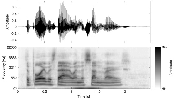
However, each of the filters will be centred on a different frequency; the frequencies vary logarithmically with the filter number (meaning that low frequency filters are much more closely spaced than high frequency filters). This is very similar to the human auditory system. The equal tempered scale also spaces notes logarithmically in order to try to match our perception of pitch (doubling a note's frequency moves it up an octave). Think of it like a graphic equaliser: each slider on a graphic equaliser corresponds to a filter (the slider controls the output gain of the filter). See the example in Fig. 1. In the lower panel, the bottom row tells you about the low frequency content of the speech signal (shown in the top panel) over time, whereas the top row tells you about the high frequency content of the speech signal over time; the darker shades show higher amplitudes.

But how is this useful to CASA? Well, we can treat this transformed version of our signal much like an image, changing individual pixels to change the sound. If we were to transform a mixture of sounds (like the mixture you hear everyday), we could reduce or eliminate some sounds by simply turning the pixels off that relate to those sounds. In practice, knowing which pixels to change is very difficult because we generally don't know anything about the sounds in the mixture: the examples in this post are made easy because we do know all of the sounds in the mixture.
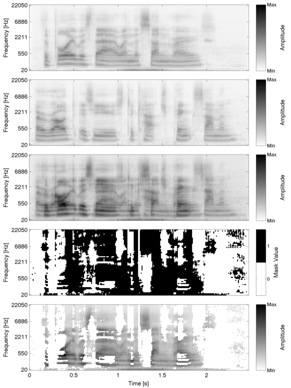
We therefore develop algorithms to calculate which parts of the sound to let through, and which parts to silence: using the terminology above, which pixels to turn on or off. If we were to display a picture of these switched pixels, it would look like the example in Fig. 2, and we call this set of switching decisions a time–frequency mask. See the example in Fig. 2. The example shows what's known as a binary mask, so called, unsurprisingly, because its values are either zero or one. Specifically, it's set to one when the sound you want (the target) is louder than the sound or sounds you don't want (the interference), and zero otherwise. All that's left to do now is to multiply the mask with the time–frequency representation of the mixture. Zero-valued elements in the mask will mute the corresponding region in the mixture, whereas unity values will leave the mixture unchanged. Then we just need to transform the result back to the time domain. Simples!
To summarise, the steps in this process are:
- Transform the mixture to the time–frequency domain.
- Calculate the time–frequency mask.
- Multiply the mask and the time–frequency mixture.
- Transform the result back to the time domain.

But I'm sure you're eager to know what this sounds like. The answer, as it happens, is not great! Listen to the examples below. Do you hear the nice bubbly artefacts? That's known as "musical noise". It's a bit like the "birdies" you sometimes hear in a low bit-rate codec (the causes are somewhat similar, too). Despite this it's still a useful technique, which is why, in collaboration with the BBC, we're currently researching this problem at the IoSR (see [4] for example). I'll talk about some possible solutions in a future blog post. The next blog post from me will be about whether the time–frequency mask should be binary OR NOT (that's an unfunny digital logic joke for the benefit of my first year Computer Audio Systems students!).
Sentence 1 (top panel, Fig. 2.)
Sentence 2 (first from top panel, Fig. 2.)
Mixture (middle panel, Fig. 2.)
Separated output (bottom panel, Fig. 2.)
References
[1] Bregman, A.S.: Auditory Scene Analysis. MIT Press, Cambridge, MA (1990).
by Chris Hummersone
